
In this case study, I analyze historical data from a Chicago based bike-share company in order to identify trends in how their customers use bikes differently. The main tools I use are spreadsheets, SQL and Tableau. Here are the highlights:
A more in-depth breakdown of the case study scenario is included below, followed
by my full report.
Scenario
Cyclistic is a bike-share company based in Chicago with two types of customers. Customers who purchase single-ride or full-day passes are known as casual riders, while those who purchase annual memberships are known as members. Cyclistic’s financial analysts have concluded that annual members are much more profitable than casual riders. The director of marketing believes the company’s future success depends on maximizing the number of annual memberships.
The marketing analytics team wants to understand how casual riders and annual members use Cyclistic bikes differently. From these insights, the team will design a new marketing strategy to convert casual riders into annual members. The primary stakeholders for this project include Cyclistic’s director of marketing and the Cyclistic executive team. The Cyclistic marketing analytics team are secondary stakeholders.
Defining the problem
The main problem for the director of marketing and marketing analytics team is this: Design marketing strategies aimed at converting Cyclistic’s casual riders into annual members. There are three questions that will guide this future marketing program. For my scope on this project, I will anlyze the first question:
1) How do annual members and casual riders use Cyclistic bikes differently?
2) Why would casual riders buy Cyclistic annual memberships?
3) How can Cyclistic use digital media to influence casual riders to become
members?
By looking at the data, we will be able to first get a broad sense of certain patterns that are occurring in the two different groups. Understanding the differences will provide more accurate customer profiles for each group. These insights will help the marketing analytics team design high quality targeted marketing for converting casual riders into members. For the Cyclistic executive team, these insights will help Cyclistic maximize the number of annual members and will fuel future growth for the company.
Business task
Analyze historical bike trip data to identify trends in how annual members and casual riders use Cyclistic bikes differently.
Data sources
We’ll be using Cyclistic’s historical bike trip data from the last 12 months, which is publicly available here. The data is made available by Motivate International Inc. under this license. The data is stored in spreadsheets. There are 12 .CSV files total:
01) 2021-02_divvy_trip-data.csv
02) 2021-03_divvy_trip-data.csv
03) 2021-04_divvy_trip-data.csv
04) 2021-05_divvy_trip-data.csv
05) 2021-06_divvy_trip-data.csv
06) 2021-07_divvy_trip-data.csv
07) 2021-08_divvy_trip-data.csv
08) 2021-09_divvy_trip-data.csv
09) 2021-10_divvy_trip-data.csv
10) 2021-11_divvy_trip-data.csv
11) 2021-12_divvy_trip-data.csv
12) 2022-01_divvy_trip-data.csv
It is structured data, organized in rows (records) and columns (fields). Each
record represents one trip, and each trip has a unique field that identifies it:
ride_id. Each trip is anonymized and includes the following fields:
* ride_id               #Ride id - unique
* rideable_type         #Bike type - Classic, Docked, Electric
* started_at            #Trip start day and time
* ended_at              #Trip end day and time
* start_station_name    #Trip start station
* start_station_id      #Trip start station id
* end_station_name      #Trip end station
* end_station_id        #Trip end station id
* start_lat             #Trip start latitude
* start_lng             #Trip start longitute
* end_lat               #Trip end latitude
* end_lat               #Trip end longitute
* member_casual         #Rider type - Member or Casual
Bike station data that is made publicly available by the city of Chicago will also be used. It can be downloaded here. In terms of bias and credibility, both data sources we are using ROCCC:
Reliable and original: this is public data that contains accurate, complete and unbiased info on Cyclistic’s historical bike trips. It can be used to explore how different customer types are using Cyclistic bikes.
Comprehensive and current: these sources contain all the data needed to understand the different ways members and casual riders use Cyclistic bikes. The data is from the past 12 months. It is current and relevant to the task at hand. This is important because the usefulness of data decreases as time passes.
Cited:these sources are publicly available data provided by Cyclistic and the City of Chicago. Governmental agency data and vetted public data are typically good sources of data.
Data cleaning and manipulation
Microsoft Excel: initial data cleaning and manipulation
Our next step is making sure the data is stored appropriately and prepared for analysis. After downloading all 12 zip files and unzipping them, I housed the files in a temporary folder on my desktop. I also created subfolders for the .CSV files and the .XLS files so that I have a copy of the original data. Then, I launched Excel, opened each file, and chose to Save As an Excel Workbook file. For each .XLS file, I did the following:
- Changed format of
started_atandended_atcolumns- Formatted as custom
DATETIME
- Format > Cells > Custom > yyyy-mm-dd h:mm:ss
- Formatted as custom
- Created a column called
ride_length- Calculated the length of each ride by subtracting the column
started_atfrom the columnended_at(example:=D2-C2)
- Formatted as
TIME
- Format > Cells > Time > HH:MM:SS (37:30:55)
- Calculated the length of each ride by subtracting the column
- Created a column called
ride_date- Calculated the date of each ride started using the
DATEcommand (example:=DATE(YEAR(C2),MONTH(C2),DAY(C2)))
- Format > Cells > Date > YYYY-MM-DD
- Calculated the date of each ride started using the
- Created a column called
ride_month- Entered the month of each ride and formatted as number (example: January:
=1)
- Format > Cells > Number
- Entered the month of each ride and formatted as number (example: January:
- Created a column called
ride_year- Entered the year of each ride and formatted as general
- Format > Cells > General > YYYY
- Entered the year of each ride and formatted as general
- Created a column called
start_time- Calculated the start time of each ride using the
started_atcolumn - Formatted as
TIME
- Format > Cells > Time > HH:MM:SS (37:30:55)
- Calculated the start time of each ride using the
- Created a column called
end_time- Calculated the end time of each ride using the
ended_atcolumn
- Formatted as
TIME
- Format > Cells > Time > HH:MM:SS (37:30:55)
- Calculated the end time of each ride using the
- Created a column called
day_of_week- Calculated the day of the week that each ride started using the
WEEKDAYcommand (example:=WEEKDAY(C2,1))
- Formatted as a
NUMBERwith no decimals
- Format > Cells > Number (no decimals) > 1,2,3,4,5,6,7
- Note: 1 = Sunday and 7 = Saturday
- Calculated the day of the week that each ride started using the
After making these updates, I saved each .XLS file as a new .CSV file.
BigQuery: further data cleaning and manipulation via SQL
Since these datasets are so large, it makes sense to move our analysis to a tool that is better suited for handling large datasets. I chose to use SQL via BigQuery.
In order to continue processing the data in BigQuery, I created a bucket in Google Cloud Storage to upload all 12 files. I then created a project in BigQuery and uploaded these files as datasets. I’ve provided my initial cleaning and transformation SQL queries here for reference: initial_setup_query.sql
The results from the COUNT DISTINCT query for each table are very interesting.
We can see that the three summer months have the highest trip counts, followed
by alternating spring and fall months before ending with winter months:
![]()
Create quarterly tables
In order to perform analysis by season, let’s combine these tables. We’ll create Q1, Q2, Q3 and Q4 tables for analysis. We’ll have two Q1 tables– one for 20221 and one for 2022 – since we have FEB/MAR data from 2021 and JAN data from 2022:
- Table 1) 2021_Q1 -> FEB(02), MAR(03)
- Table 2) 2021_Q2 -> APR(04), MAY(05), JUN(06)
- Table 3) 2021_Q3 -> JUL(07), AUG(08), SEP(09)
- Table 4) 2021_Q4 -> OCT(10), NOV(11), DEC(12)
- Table 5) 2022_Q1 -> JAN(01)
We’ll first create 2021_Q2 and then repeat for the remaining four tables:
Clean and transform day of week
Some additional data cleaning is needed on the new table. First, we’ll update
the format for day_of_week from FLOAT to STRING. Then, we’ll change the
values from numbers to their corresponding day names (i.e. 1 = Sunday, 7 =
Saturday. We’ll start with 2021_Q1 and repeat for the remaining four tables:
Delete old tables
Now that we have our tables organized into quarters, we can delete the original monthly tables from BigQuery. We no longer need the monthly tables since the data is available in the quarter tables. Also, it costs money to store these datasets in BigQuery.
Analysis #1: Exploratory
2021_Q1 - quarterly data exploration
We’ll select a few columns from 2021_Q1 to preview in a temporary table. This will help give us an idea of potential trends and relationships to explore further:
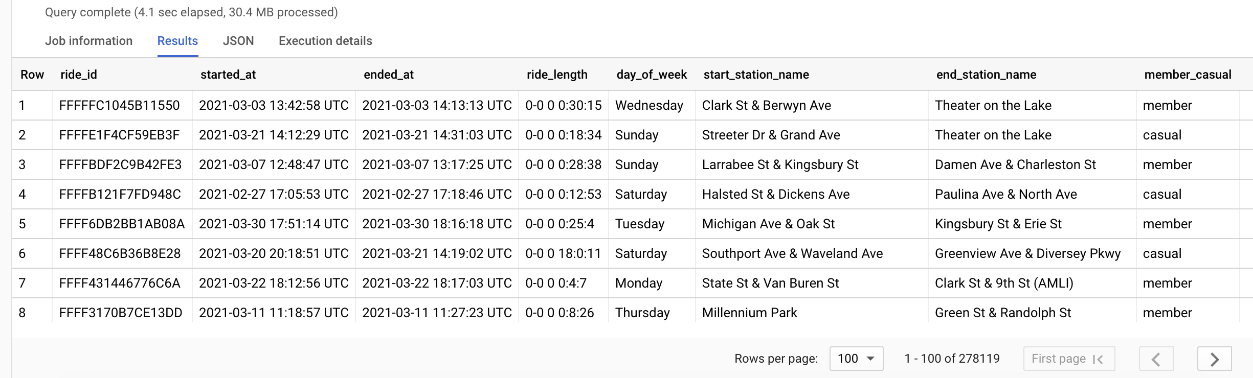
The above query returned 278,119 rows. That is the number of recorded trips we have data for in this quarter. Let’s dive deeper into those trip totals.
Total trips
We’ll create total columns for overall, annual members and casual riders. We’ll also calculate percentages of overall total for both types:
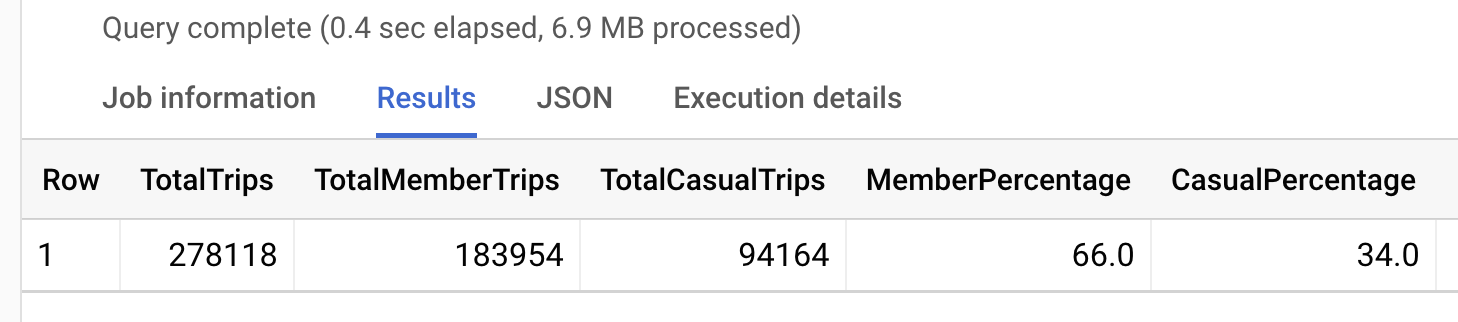
Of the 278,118 total trips in 2021_Q1, 66% were from annual members while 34% were from casual riders.
Average ride lengths
How does average ride_length differ for these groups?
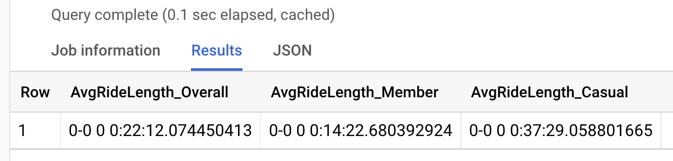
We can see that casual riders average about 23 more minutes per ride. That seems like a pretty big difference. What influence are outliers having on these averages? Let’s investigate.
Max ride lengths
We’ll look at the maximum values for ride_length to see if anything extreme is
influencing the casual rider average:
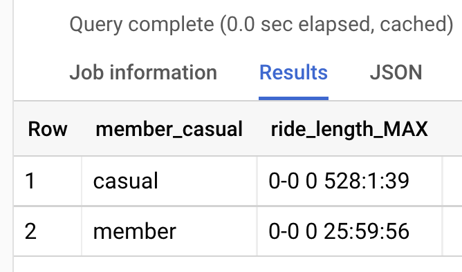
As we suspected, the casual riders average ride_length was significantly
impacted by at least one outlier. The longest trip duration for casual riders
was 528 hours, or 22 days. Meanwhile, the longest for annual was about 26 hours.
Let’s take a look at the top 100 highest ride_length values for casual riders
to confirm there is more than one outlier affecting the average:

Median ride lengths
Since there are more than a few outliers impacting the average, we’re going to use median instead of average. Median will be more accurate for our analysis:
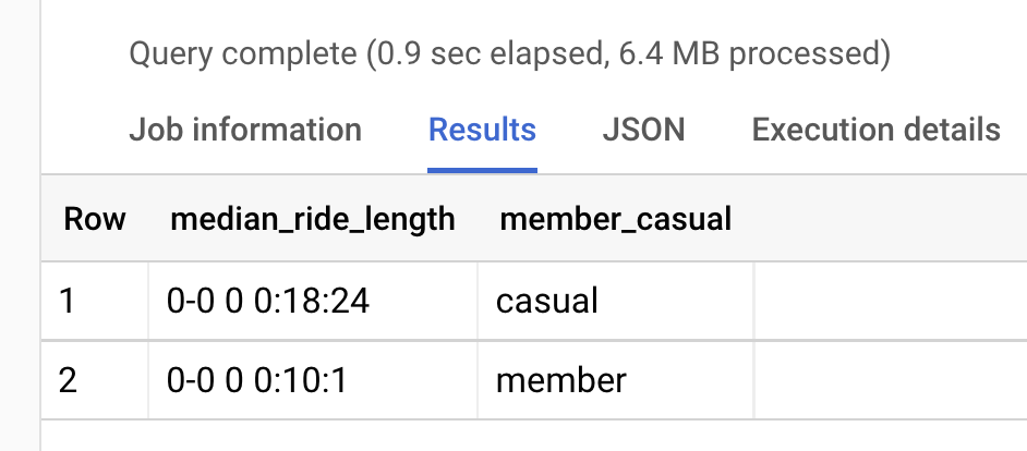
Now we see a much closer number, with 18 minutes for casual riders and 10 minutes for annual members.
Busiest day for rides
Let’s see which day has the most rides for annual members and casual riders:
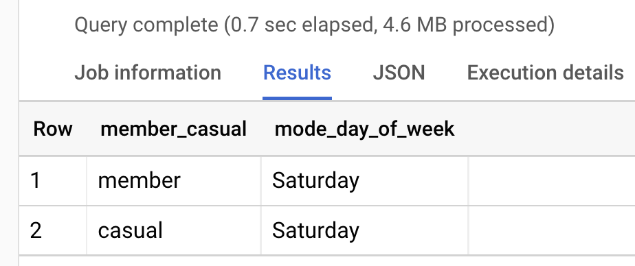
Unsurprisingly, Saturday is the most popular day for both annual members and casual riders.
Median ride length per day
Let’s look at the median ride lengths per day for both annual members and casual riders. Since Saturday is the most popular overall, do we think it will also have the highest median ride length?
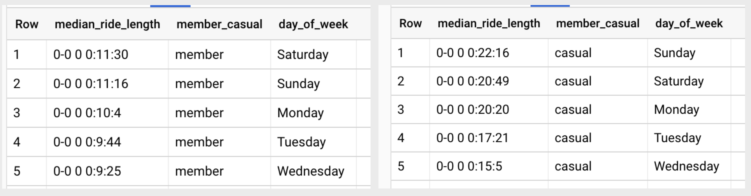
Very interesting! The median ride length for casual riders on the top five days (SUN, SAT, MON, TUE, WED) is nearly double the amount for annual members on their top five days (SAT, SUN, MON, TUE, WED).
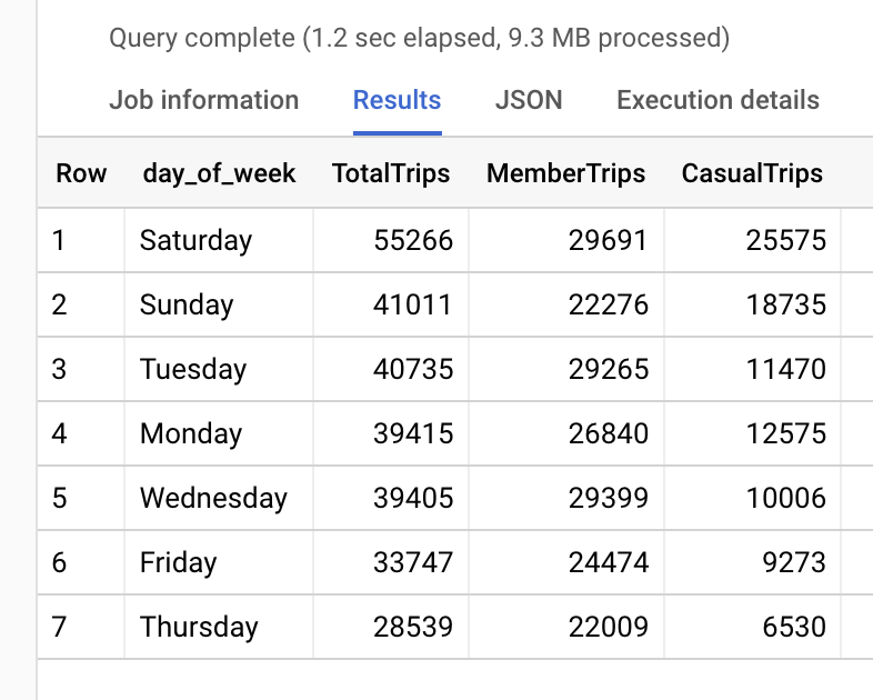
Total rides per day
Let’s look at total rides per day. We’ll create columns for overall total, annual members and casual riders:
Start stations
Next, we’ll look at the most popular start stations for trips. We’ll again include columns for overall, annual member and casual rider totals per start station:
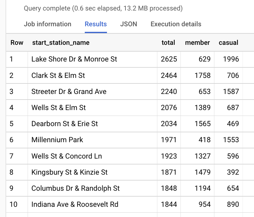
We can begin to see some interesting patterns in the start station data. It
looks like casual riders and annual members tend to favor different regions
for beginning their trips. By updating the ORDER BY function to sort by
casual DESC and member DESC in two separate queries, we can compare the
top ten start stations for both:
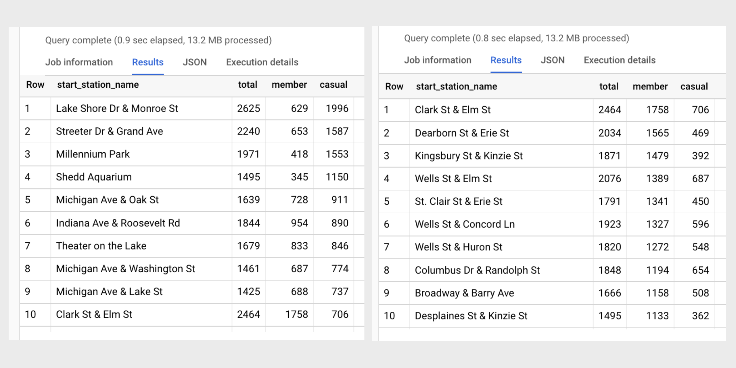
Wow! There is only one start station that cracks the top ten for both lists.
The Clark St & Elm St
start station is ranked #1 for annual members and #10 for casual riders. The
casual riders seem to favor stations near the water like Lake Shore Dr & Monroe St and Streeter Dr & Grand Ave, while
annual members frequent start stations in the River North neighborhood like
Dearborn St & Erie St
and Kingsbury St & Kinzie St.
An initial hypothesis for casual riders could be that they tend to favor start stations near the water and close to tourist attractions because they use bikes for weekend entertainment. An initial hypothesis for annual members could be that they tend to favor start stations in downtown, retail areas because they are using bikes for their work commutes and shopping trips.
Quarterly data exploration (cont.)
Instead of walking through each quarter like we’ve done for 2021_Q1, I will instead provide links to the full SQL files. The queries used are similar to the ones above:
- analysis_2021_Q1.sql
- analysis_2021_Q2.sql
- analysis_2021_Q3.sql
- analysis_2021_Q4.sql
- analysis_2022_Q1.sql
I’ll included some high-level quarterly analysis notes in the next section.
Analysis #2: Summary
full_year - trends, relationships and insights
In order to analyze all twelve months together, we’ll combine the five quarterly tables into one table. The queries used to accomplish this are included here for reference. I’ve also provided the SQL file used for full year analysis: analysis_full_year.sql.
For a summary and overall visualization of my full year analysis, please visit the
Tableau Public dashboard I created here: Tableau Dashboard: Cyclistic Bikeshare in Chicago.
I will also highlight some of the interesting trends and relationships I discovered
below.
Annual Members vs Casual Riders
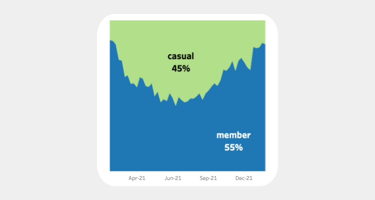
During the past 12 months, annual members accounted for 55% of Cyclistic’s total
trips while casual riders accounted for 45% of total trips. As we can see in the
above area chart, this percentage fluctuates throughout the year.
Seasonal trends

Summer vs Winter
The busiest time of year for overall bike trips is Q3– July, August and September. This makes sense because these months are mainly summer time. Bike riding is better suited for warmer weather, which is also why we see a major drop-off in total rides during the winter months of Q1– January, February and March.
Annual members outnumbered casual riders in every quarter except Q3. Interestingly, the annual members nearly doubled the casual ridership in Q1 and Q4 while only slightly edging them out in Q2.
Median ride length
We learned in the earlier quarterly analysis that the average ride_length for
casual riders was significantly impacted by outliers, so median is a more
accurate measurement for our analysis:

We can see that casual riders consistently have longer rides than annual members.
Day of week
Which days of the week have the highest number of rides for casual riders vs annual members? Let’s look at the mode for each quarter and for the full year:
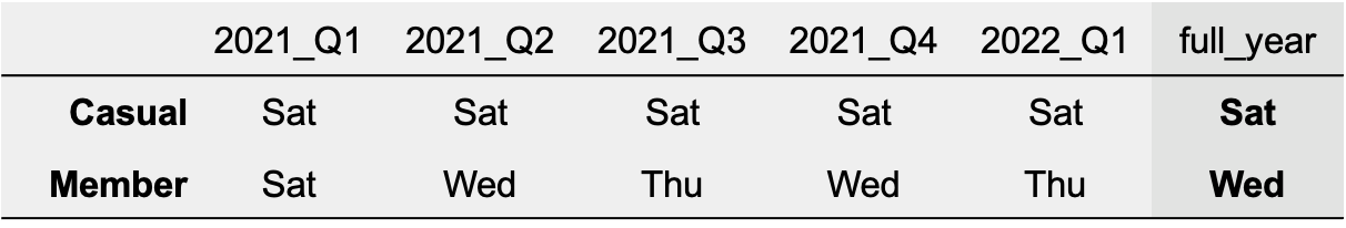
Casual riders were extremely consistent, with Saturday revealing itself as their preferred day of week for each quarter and across the full year. Meanwhile, the annual members looked to favor the middle of the week for their bike use. The most popular day for them acrosss the full year was Wednesday. Let’s see how the total rides for each day stack up for both groups:

How about median ride length per day of week for both groups?

A few fascinating insights from the above chart:
U-shape pattern
Sunday and Saturday are favored by both groups for longer rides, while ride duration decreases towards the middle of the week before increasing again on Friday. This results in a u-shape trend for both groups in the above chart, although it is much more dramatic for casual riders.Range differences
For annual members, difference between their longest day and their shortest day is 1 minute and 44 seconds. For casual riders, difference is 4 minute and 57 seconds. That is a 185.58% increase in difference for casual riders.Annual members: day-to-day consistency
The annual members may have shorter ride lengths when compared to casual riders, but they are extremely consistent with their bike use day-over-day.Casual riders: weekend warriors
The daily median ride length for casual riders is consistently higher than that of annual members. The range of their ride length duration varies at a greater amount than that of annual members. Sundays and Saturdays stand out as their longest ride days.
Bike type
Do members and casual riders have different preferences for bike type? Are classic bikes more popular than electric bikes?

We can see that classic bikes are favored by both groups. Let’s look at the percentages of bike type use within each group:

Looking at the above, we might ask what exactly is a docked bike and why are only casual riders using them?
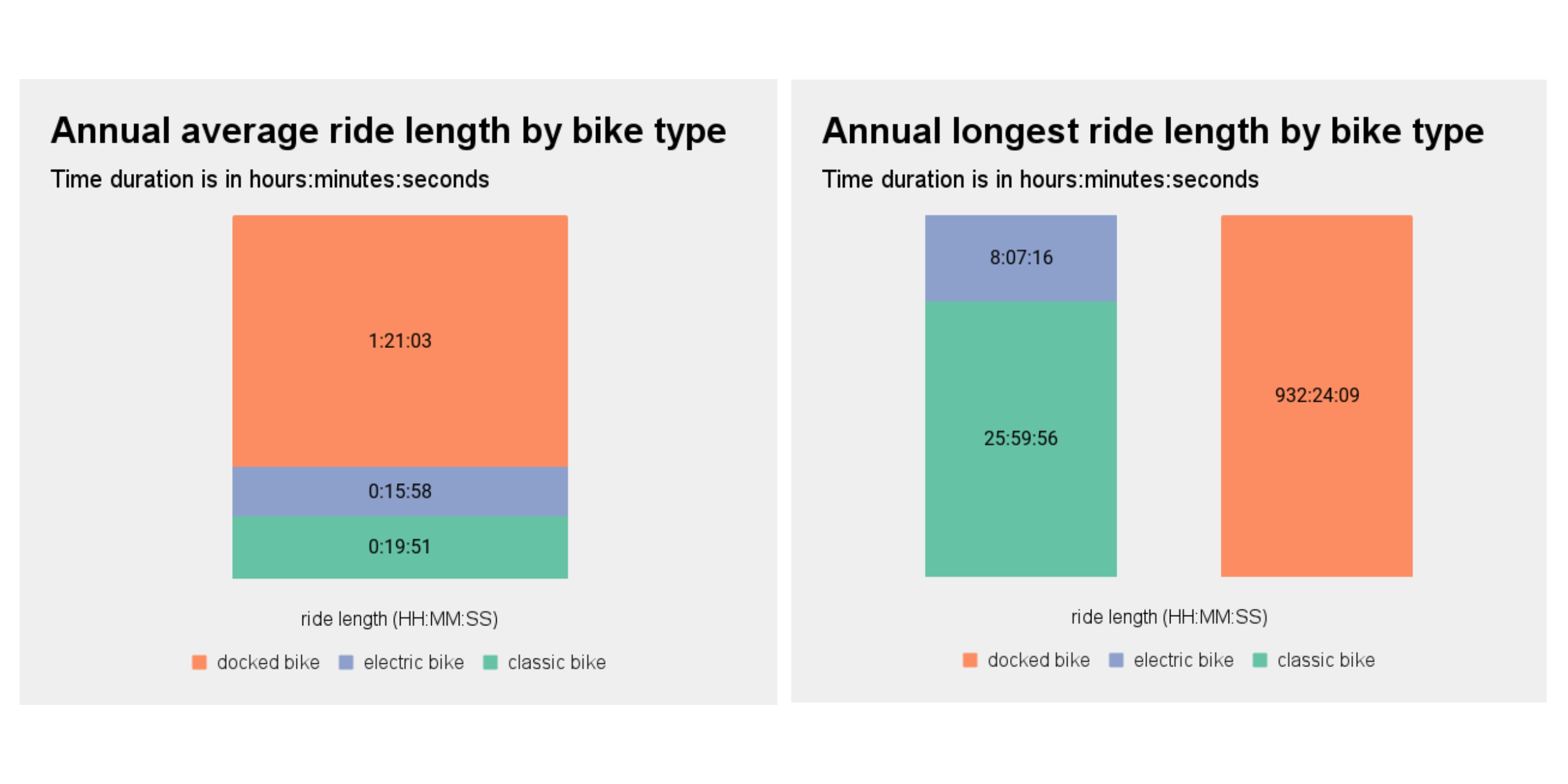
We can now see from the above charts that docked bikes are the culprit for the outliers affecting our ride length averages from earlier in our analysis. This is something we should discuss with our team further and address.
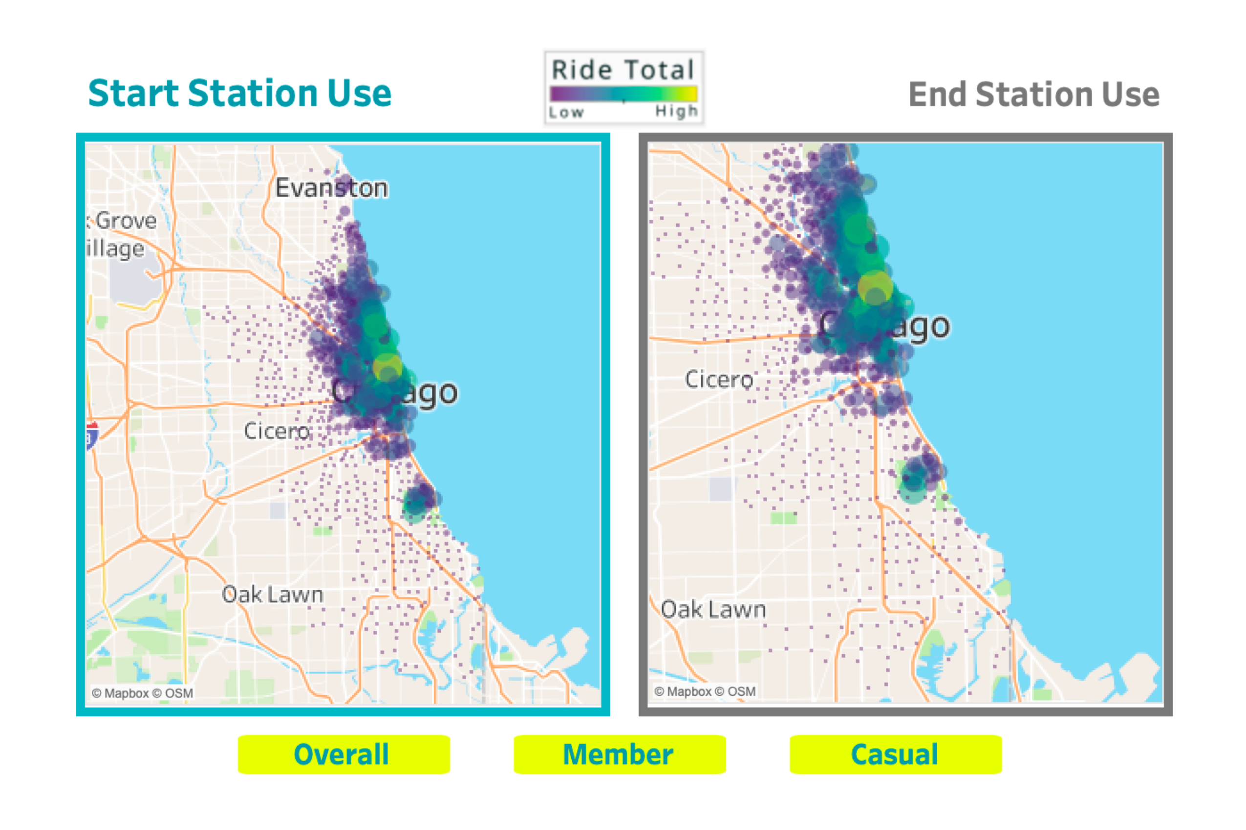
Start and end station use
In the Tableau Dashboard I created, which is again available here, there is a worksheet that allows the exploration of start and end station use by members, casual riders and combined overall rides. The snapshot below is from the overall view. While interacting with the dashboard, we can see that casual riders have a higher max than annual members. Annual members have a lower max, but we can see more colors represented across the member map versus the consistent coloring across the casual map. This tells us that rides by members are more distributed across stations while rides by casual riders are more top heavy in that a huge chunk are happening at the same few stations.
Conclusion
Stakeholder presentation and dashboard
I’ve provided links below for my dashboard and shareholder presentation, which includes the following:
- A summary of my analysis
- Supporting visualizations and key findings
- Three recommendations based on my analysis
Presentation: Where Rubber Meets Road in Converting Casual Riders to Cyclistic Members